Resolving Rule Conflicts with Log-Linear Sum
Basic Idea
The Log-Linear formula is adopted from the Logistic Regression method. Let vector R be the set of induced unordered rules {R1, ..., Rn} and let x be an example we would like to classify. The Log-Linear model for rule classification in two-class domains (c0, c1) is a weighted sum (W is a real-valued vector):
| |
|
| |
| |
|
| w0+w1×R1(x) + ...+ wn×Rn(x), |
| | (5) |
|
where weights w1, ... , wn given to rules are all nonnegative reals. The terms Ri(x) are defined as:
|
Ri(x) = |
|
|
|
|
|
|
| |
if conditions of Ri are false for example x; |
|
| |
| |
|
|
| (6) |
The predicted probability of class c1 for example x is computed from f(x) through the logit link function:
Although this particular model can only be used in domains with two classes, it can be extended to its multi-class version, in the same way as basic logistic regression is extended into a multinomial logistic regression.
Using log-linear sum for rule classification is implicitly already used in Naive-Bayesian classification from rules. However, Naive Bayes assigns weights to each rule independently from other rules, which can be a problem if the rules are correlated. And they usually are! I propose a different way of doing it. I demand that the log-linear model gives predictions that are consistent with predictions of single rules, which automatically assures that correlated rules will not bias the model.
Implementation in Orange
This classification method is implemented within the Orange data-mining software, which you can download from http://www.ailab.si/orange/downloads.asp. I propose taking the latest snapshot, as Orange is getting better every day.
The class orngCN2.CN2EVCUnorderedLearner combines EVC evaluation of rules, probabilistic covering and LCR classification. This learnRules.py script illustrates how rules can be learned and printed along with their coefficients. The learnRulesParams.py is a script that describes all possible parameters accepted by CN2EVCUnorderedLearner and demonstrates how these parameters could be changed. For the above script, you will need the well-known Titanic data-set.
Visualisation
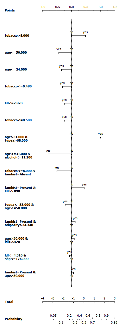
Obtained rules can be visualised with the standard widget for presenting rules in Orange, see rulesWidget.py as an example how to do it. Moreover, the log-linear formula also allows a nice visualisation with nomograms, which are usually used for logistic-regression and linear models alike. The nomogram.py script shows how rules can be submitted to nomograms widget. You will need the SAHeart data-set. The obtained nomogram is shown in the picture below-left, while rules in widget are in the image to the right. In nomogram, each horizontal line corresponds to one rule. The conditions of the rule are described as text at the left. The value yes on the line denotes the rule contribution if it triggers for the example, otherwise its contribution is zero. The nomogram nicelly shows how a rule is relevant with respect to other rules; for example, the age>31 and type>68 rule has a much lower accuracy than tobacco<0.480, however it has a considerably larger weight, as the "tobacco" rule must be explained already by other rules.
 |  |